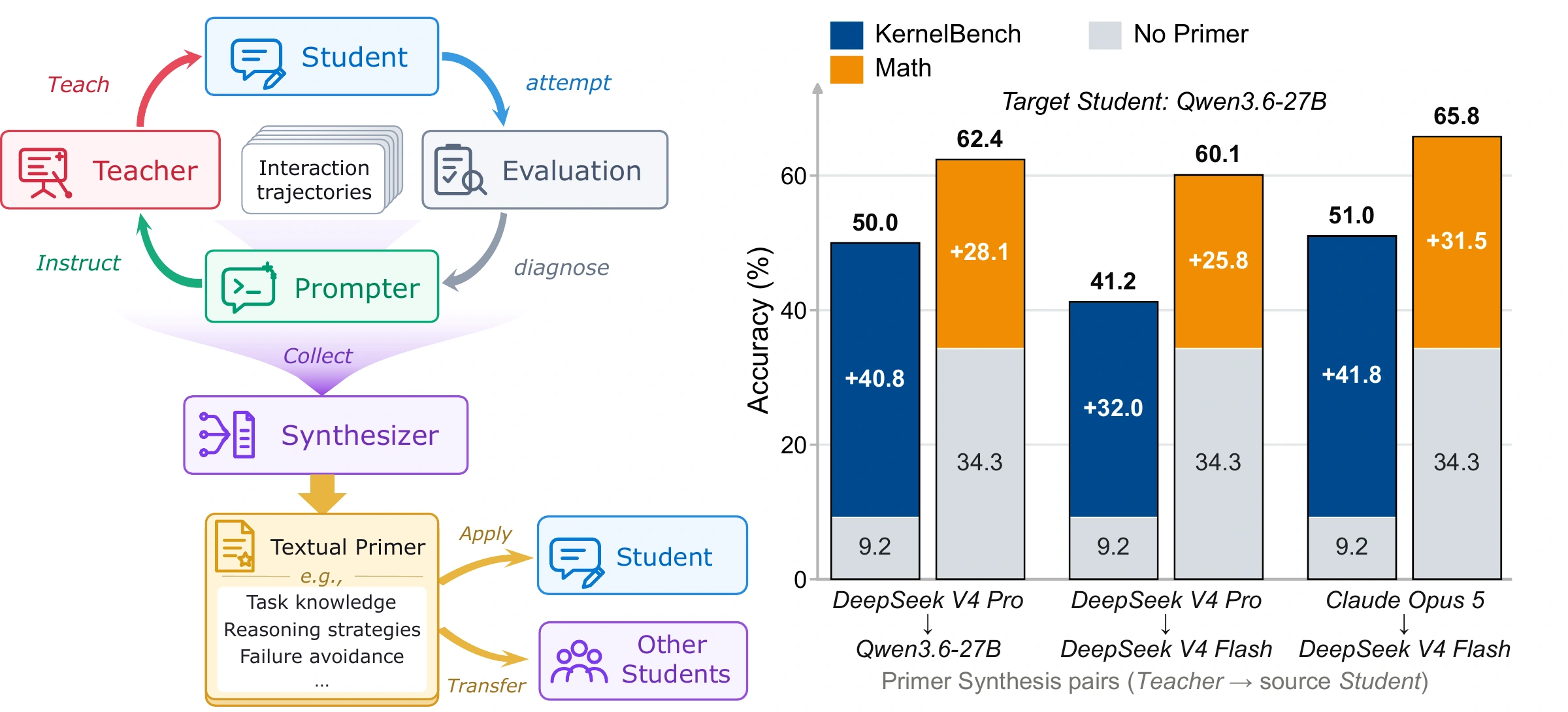
Universal Textual Teaching (UTT) distills an LLM’s knowledge into a textual Primer through multi-role interactions. The Primer improves its source Student and transfers to other Students without resynthesis. When Qwen3.6-27B does not participate in synthesis, accuracy gains reach 41.8 and 31.5 percentage points on KernelBench and Omni-MATH-2, respectively.
Abstract
Knowledge distillation (KD) transfers knowledge from stronger Teacher models to weaker Student models, but most methods require training the Student parameters, thereby binding the distilled knowledge to a specific architecture and checkpoint. This implicit representation is difficult to interpret or reuse across models and limits KD for API-only or costly-to-train models. This paper studies knowledge transfer for large language models (LLMs). We introduce Universal Textual Teaching (UTT), a parameter-update-free framework that distills observed Teacher–Student knowledge gaps into a textual, interpretable, and reusable natural-language artifact called Primer.
Specifically, UTT first identifies representative gap cases through paired evaluations, and iteratively updates the Primer via multi-role interactions: the Student attempts each task, the Prompter turns evaluation feedback into a teaching instruction, the Teacher provides a targeted demonstration, and the Synthesizer consolidates validated lessons. Empirically, on the challenging math (Omni-MATH-2) and code generation (KernelBench) tasks, extensive results confirm the effectiveness of the method: UTT remarkably raises the Student’s accuracy from 9.4% to 48.6% and Fast₁ accuracy from 9% to 35% on KernelBench, while increasing mathematical reasoning accuracy from 27.6% to 51.7%. UTT also performs better than representative prompt engineering and parameter-based KD methods. Of note, UTT is shown to be generalizable across different Teachers and Students: a Primer synthesized for one Teacher–Student pair can generalize to other Students that do not participate in the synthesis.
Overview of our UTT method
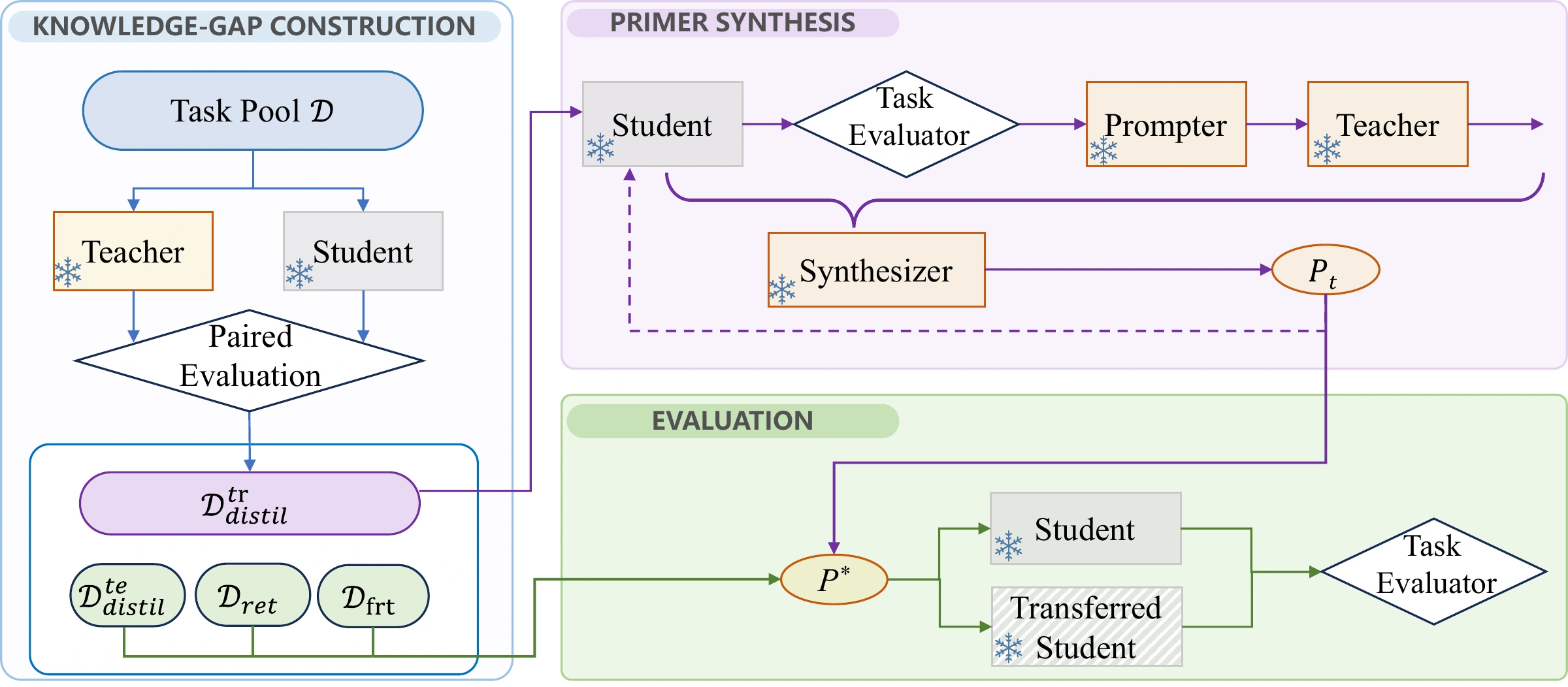
Illustration of the proposed UTT framework. Paired evaluation identifies Teacher–Student knowledge gaps. The Student attempts each task; the Prompter diagnoses feedback; the Teacher provides a demonstration; and the Synthesizer consolidates validated teaching records. Candidate Primers are accepted when accuracy on the current batch does not decrease. All model parameters remain fixed.
The Teacher model also serves as the Prompter and Synthesizer. The final Primer is prepended to task inputs and can be reused by another Student without resynthesis.
Main Results
Primer effectiveness and cross-model transferability
Primer synthesis
Target Student
Teacher
Teacher score
Source Student
Flash
Qwen
KernelBench Accuracy (%)
No Primer
9.4
9.2
Pro
19.6
Flash
48.6 (+39.2)
41.2 (+32.0)
Pro
19.6
Qwen
43.8 (+34.4)
50.0 (+40.8)
Opus
36.0
Flash
48.2 (+38.8)
51.0 (+41.8)
KernelBench Fast₁@5 (%)
No Primer
9
12
Pro
20
Flash
35 (+26)
37 (+25)
Pro
20
Qwen
30 (+21)
32 (+20)
Opus
41
Flash
39 (+30)
22 (+10)
Omni-MATH-2 Accuracy (%)
No Primer
27.6
34.3
Pro
51.4
Flash
51.7 (+24.1)
60.1 (+25.8)
Pro
51.4
Qwen
43.7 (+16.1)
62.4 (+28.1)
Opus
92.5
Flash
46.6 (+19.0)
65.8 (+31.5)
Table 1. For each task, each Teacher and source Student pair produces one Primer, which is applied to both target Students. Parentheses show gains in percentage points over the corresponding baseline. The best score for each target Student and metric is in bold.
Comparison with prompt engineering methods
Method
Omni-MATH-2 accuracy
KernelBench · Flash
KernelBench · Qwen
Flash
Qwen
Accuracy
Fast₁@5
Accuracy
Fast₁@5
Student · no Primer
27.6
34.3
9.4
9
9.2
12
One-shot
35.0
57.7
39.2
23
45.8
31
Few-shot
35.4
54.8
40.6
25
46.6
30
Teacher summary
36.7
32.8
40.0
30
10.2
11
APE
31.0
39.3
11.0
8
10.4
13
MIPROv2 · instruction only
28.7
29.8
9.8
6
11.8
9
MIPROv2
33.5
25.8
45.0
21
44.6
30
GEPA
41.1
61.9
34.8
24
32.6
23
UTT (Ours)
51.7
62.4
48.6
35
50.0
32
Table 2. UTT achieves the best reported score across all six model–metric combinations in this comparison. “Teacher summary” asks the Teacher to summarize the training set into a general prompt. All values are percentages.
Comparison with knowledge distillation methods
Method
Omni-MATH-2 accuracy (%)
KernelBench accuracy (%)
KernelBench Fast₁@5 (%)
Student · no Primer
34.3
9.2
12
SeqKD
53.5
18.8
18
Fine-tune-CoT
39.5
41.8
28
RSR
51.5
22.6
19
LUFFY
55.2
11.4
13
UTT (Ours)
62.4
50.0
32
Table 3. Results under the Pro → Qwen setting. KD baselines train LoRA adapters on a frozen Qwen backbone; UTT updates no model parameters. All methods use the same distillation-training problems.
1 / 3
Models. Pro: DeepSeek V4 Pro; Flash: DeepSeek V4 Flash; Qwen: Qwen3.6-27B; Opus: Claude Opus 5.
More Results and Analysis
Extension to multimodal reasoning
100 visual geometry problems from the Vision Dominant subset of MathVerse, with two responses per problem.
Primer synthesis
Target Student
Teacher
Teacher score
Source Student
Flash 4.1
Qwen
MathVerse Accuracy (%)
No Primer
54.0
41.5
Max
94.0
Qwen
59.0 (+5.0)
76.0 (+34.5)
Max
94.0
Flash 4.1
56.0 (+2.0)
72.0 (+30.5)
Opus
93.5
Qwen
57.5 (+3.5)
80.5 (+39.0)
The Primer improves every source and transfer Student. Qwen accuracy reaches 80.5% with the Opus → Qwen Primer; transferring the Max → Qwen Primer to Flash 4.1 raises accuracy from 54.0% to 59.0%. Parentheses show percentage-point gains over each target Student’s baseline; bold values mark the best result for each target Student.
Models. Max: Qwen3.8-Max; Qwen: Qwen3.6-27B; Flash 4.1: DeepSeek-V4.1-Flash; Opus: Claude Opus 5.
Generalization, retention, and frontier extension
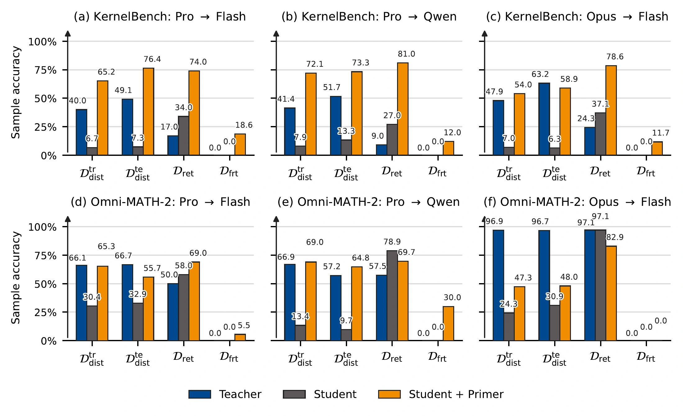
Split-wise sample accuracy. On the held-out Omni-MATH-2 distillation-test subset, Pro → Qwen improves from 9.7% to 64.8%. Retention is not uniform: math retention accuracy decreases by 9.2 and 14.2 percentage points for Pro → Qwen and Opus → Flash, respectively.
Primer effectiveness under larger token budgets
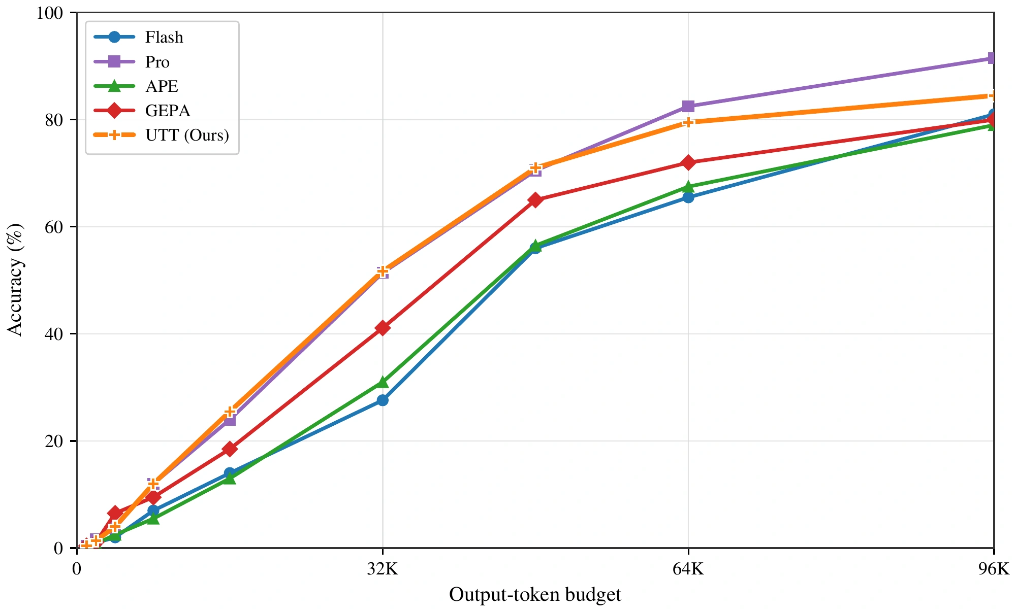
The Primer synthesized at the 32k budget is reused without resynthesis at larger budgets. At the largest tested budget, UTT remains above the unprimed Student and below the Teacher.
1 / 3
Primer Examples
Full examples of the generated Primers for mathematical reasoning, GPU kernel generation, and multimodal geometry.
End with a finite checkable proof/boxed answer; prefer compact algebra, counting, or graph arguments.
Verify definitions, boundary cases, and small examples before trusting analogies or known results.
1 Geometry
Circle tangency via coordinates: normalize; circle through points x2+y2+ax+by+c=0; prove common point and proportional gradients.
Billiards by unfolding: reflect polygon, not ray; path becomes straight segment in tiling; use gcd/color conditions for vertex hits.
Distinguish metric vs combinatorial definitions; use explicit polar/nonregular counterexamples.
Tetrahedron altitude from six edges: build base B′C′D′; build rotated face points AB opposite side of C′D′ with ABC′=AC,ABD′=AD, and AC opposite side of B′D′ with ACB′=AB,ACD′=AD. Perpendiculars from AB to line C′D′ and AC to line B′D′ meet at the true foot X′. Altitude =∣ABY′∣2−∣X′Y′∣2, constructible by Pythagorean difference. Use full supporting lines, not segments. Foot from A to line BC has signed BP=(AB2+BC2−AC2)/(2BC); BP<0 or BP>BC means foot outside segment. Transfer signed positions; unsigned distances fail in obtuse cases.
2 Number theory and polynomial values
2.1 Vieta jumping/descent
For (a+b)(a+b+1)/(ab)=N: fix N, rewrite as quadratic, Vieta gives positive integer other root; descend to equal pair; verify integrality/positivity.
2.2 Lyndon words and fractional parts
Suffix/prefix lex conditions become Lyndon words; count length L over q by L1∑d∣Lμ(d)qL/d.
2.3 Reduced denominators / averaging
For Sn=An/n!, denominator n!/gcd(An,n!); lifts Ar+pk≡Ar−pk(modpk+1); existence via averaging and Stirling.
2.4 Sum-of-k-others and omitted elements
If each element is a sum of k others in a set of k+m, count omitted elements; compare largest/smallest omitted sums. Don't use sign-count bounds: largest need not be positive sum. For zero-sum symmetric sets solve a+b+c=−2x.
At x=i, analyze vπ((ki))=vπ(Nk/k!). For p≡1(mod4), p=ππˉ in Z[i]; Hensel gives s with πe∣i−s, so among i,…,i−k+1 at least ⌊k/pe⌋ are divisible by πe; hence no p≡1(mod4) appears in denominators.
p=2 or p≡3(mod4) attainable: 1/2=6(4x)+3; 1/p=(p−1)!(px).
Answer: a+bi, a,b∈Q, with νp(a),νp(b)≥0 for every p≡1(mod4). Not all Q(i): 1/5 excluded.
2.7 Prime-divisor constraints ω(n)>K
Strict >K means minimal ω(n)=K+1; constants c need c>0, ω(c)≤K+1. Boundary ω(c)=K+2 with ω(n)=K+1.
Monomials xm work.
Nonconstant nonmonomials fail. If P(0)=0, Schur gives K+2 primes qi with nonzero roots aimodqi; CRT+Dirichlet builds n with exactly K+1 prime factors and n≡aimodqi; then qi∣P(n), qi∤n, so ω(P(n))≥K+2 or P(n)≤0. If P(0)=0, factor xmQ(x), Q(0)=0, apply to Q; handle constant factor c>1.
3 Scheduling and exact-degree constructions
Tournament stays: interval per player; pairwise intersection + Helly gives common day; one match at central day; total cost baseline 2M plus idle player-days; balance distinct players before/after.
Touch/degree: for n objects each touching exactly 3 others, handshake gives 3n even, so n even; do not infer divisibility by 4. For large even n, cycle base (outside squares on 4m-gon plus reflected pairs gives 6m) and insert four-square gadgets at cuts to add 8 or 16, covering residues mod 6; verify no unintended intersections.
4 Hamiltonian paths on grids
Numbering an n×n grid is a Hamiltonian path; diagonal projection gives a ±1-walk, main diagonal visits same parity. Bound first/last visits using side color counts; construct explicitly.
5 Permutation reachability via swap graphs
Allowed swaps = graph edges; connected graph iff every permutation reachable. Prove connectivity by explicit spanning path; disprove by separated component.
6 Local block constraints and two-stage counting
Count distinguished positions first, then assign remaining; encode as 0,±1. For 2×2 zero-sum blocks, general solution aij=(−1)i+j(ri+cj); propagate sign choices across overlaps.
7 Hyperplane-generic finite sets
Minimal k-generic sets: lower via concurrent lines with k points; upper via private-point subcover and affine linear functions; incidence/basis gives ∣M∣≤kn for k,n>1.
8 Partition minima and smoothing
Define S(N)=minn1+⋯+nm=N∑f(ni) for nonincreasing f. Balanced partition is only an upper bound: S(N)≤rf(q+1)+(m−r)f(q), N=mq+r, 0≤r<m. Summing one fixed partition family overcounts because S is the minimum over all partitions. Count all zero parts: for m=20, N=0,…,19, coefficient of f(0) is 20+⋯+1=210, not 20.
Smoothing extremal: if ∑f(i)=A=(2a+1), then ∑N≥0S(N)≤∑N=0ma(ma−N)=ma(ma+1)/2. Equality at f(i)=max(a−i,0), g(N)=max(ma−N,0). Verify: f(ni)≥a−ni, so sum ≥ma−N, and sum ≥0.
9 Fair bounded selection with biased coins
Do not assume arbitrary outcome probabilities can be partitioned into n equal groups. For n=3, p=1/3, L=3, weights 8,4,4,4,2,2,2,1 cannot split into three sums 9 (8 must pair with 1; remaining even weights cannot sum 9).
Verified construction: choose p1=1/n, p2=1/2; take c with N=2c≥n(n−1), announce L=c+1. Toss coin1 once, coin2 c times. In units 1/(nN), there are NT-outcomes of weight n−1 and NH-outcomes of weight 1; each person needs total weight N. Write N=qn+r, 0≤r<n; set ai=q+1 for r people, ai=q otherwise; bi=N−ai(n−1). Feasibility ai(n−1)≤N follows from N≥n(n−1). Assign aiT-strings and biH-strings to person i; probability ai(n−1)/(nN)+bi/(nN)=1/n. Explicitly verify the partition before announcing.
PRIMER: Writing Custom CUDA Operators for PyTorch Models
Core Requirements
Replace operators with a custom CUDA implementation, typically inside a torch.autograd.Function or as a direct extension function.
Notry/except or fallback logic — let assertions crash.
Output format is critical: the entire answer must be raw Python source, starting with the first character and continuing until the end. If the instruction says “output only the code,” the response must be solely the code block—no introductory or trailing text and no Markdown fences.
All methods must be fully implemented, with no placeholders.
Token Budget & Code-First Strategy
Code output must come immediately. Spending the budget on reasoning before the code can lead to truncation, leaving no answer at all.
Prefer a minimal, correct kernel, such as one thread per output element or a serial scan, to remain within the token limit.
For inference-only tasks, skip backward computation by raising NotImplementedError.
Target roughly 60–80 lines of model code; simplify kernels that grow substantially larger.
Symbol Visibility Before Binding (Critical)
Every function referenced by m.def must be known at the point of registration. The extension binding code is a plain C++ translation unit and does not permit linking later to unresolved symbols. Two safe patterns are:
Monolithic source (recommended): define all functions before the PYBIND11_MODULE block inside a single CUDA source string and leave cpp_sources=[].
Multi-file: declare the wrapper function in a header included by the binding file. Its definition in a separate .cu file must exactly match the declaration.
The host function signature must be compatible with torch::wrap_pybind_function, conceptually a std::function accepting the specified argument types and returning a torch::Tensor. Using &my_func directly is simpler and preferred.
One thread per output for convolution, pooling, and similar operations: launch one thread per output element, loop over kernel and channel dimensions, and use __ldg for read-only data.
Scan-type operations such as cumulative sums: default to one thread per independent slice, looping sequentially over the scan dimension. This is simple, token-efficient, and reliable.
Reverse cumulative sums: loop from right to left rather than composing flip, cumulative sum, and another flip.
Multidimensional indexing: parenthesize expressions aggressively to avoid compilation failures caused by missing parentheses.
Implementing Scan Operations
Treat the tensor as (num_vectors, L), moving the target dimension to the final position when necessary.
Launch num_vectors threads, each performing a serial inclusive scan.
For a reverse cumulative sum, iterate from right to left.
Let the host wrapper move the target dimension to the end, launch on a two-dimensional view, and permute the result back.
Extension Building with load_inline
Exactly one PYBIND11_MODULE must appear, with TORCH_EXTENSION_NAME as its first argument.
The name supplied to load_inline must match the module name represented by the macro.
Use extra_cflags=["-O3"] and extra_cuda_cflags=["-O3"].
Compile once and cache the module at the class level to avoid recompilation for every instance.
Lazy Compilation (Class-Level Caching)
class ModelNew(nn.Module):
    _ext = None
    def __init__(self, dim):
        if ModelNew._ext is None:
            ModelNew._ext = load_inline(
                name="op",
                cpp_sources=[],
                cuda_sources=[cuda_src],
                verbose=False)
        self.ext = ModelNew._ext
Testing Builds Locally
Verify that a small extension compiles and executes before integrating it:
One letter is the deliverable. Write "Answer: X" first (or end with the bare letter on its own line), then 2–6 lines of justification. Nearly every observed failure was identical: no final output — budget burned re-reading the figure, cataloguing every labeled value, or debating which vertex owns a number. Partial reasoning scores zero; a best guess always beats silence.
Budget policy: 2–4 reasoning steps, at most one or two figure interpretations, then stop.
Value matches an option → commit; stop verifying.
Matches nothing → say so in one sentence, switch the assignment once, else pick the nearest listed value.
Never solve for every lettered unknown; stop the instant the target is pinned.
"Cannot be determined" only after a determinate chain visibly breaks — never as a hedge.
1. Read the figure, then isolate one unknown
Attach each number to the vertex/side/bracket its mark touches; name it ("∠MLJ=30∘"). An arrow from a value just labels the adjacent lettered angle (r∘←90 means r=90).
Decide what each length denotes: radius vs diameter, whole bracket vs sub-segment, side vs apothem, slant vs height. Label-swapping is the #1 distractor generator. An arrow drawn inside a small circle from its center is that circle's radius.
List only the structural facts you need: which point-triples are collinear, which segments are parallel/tangent.
Chain, don't systematize: anchor on the triangle/relation with two knowns, propagate, stop.
Prune decoys explicitly; extra labels often serve other sub-questions.
Not-to-scale figures: test candidate readings against options; keep the clean one.
2. Angle propagation toolkit
Two tools carry most crossing-line figures: vertical angles at the intersection and 180∘ sums (triangle, straight angle). Template: triangle with two given angles → third angle → vertical angle across → next triangle → straight-angle subtraction → target.
Parallel lines: arrowheads declare the parallel pair; find the transversal joining target to given. Corresponding/alternate interior ⇒ equal; co-interior or linear pair ⇒ supplementary. Misreading same-side as alternate gives the 180−θ distractor. Extended ray ⇒ linear pair. In a parallelogram a diagonal is a transversal for both side pairs; pair the correct halves. Quadrilateral interior sum 360∘.
3. Congruent/joined figures
Congruent polygons glued along a shared side: corresponding angles transfer; the angle at a seam vertex is usually the sum of one angle from each. Validate with polygon angle sums.
4. Similar triangles (parallels, shadows, mirrors)
AB∥CD with apex P⇒△PAB∼△PCD; h(P→AB)=(AB/CD)⋅h(P→CD). Distance between parallels =htotal−hsub (must be < total). Mirror/shadow: hfar/hnear=dfar/dnear.
5. Circle toolkit
Find diameters first: collinear labeled points through the center ⇒ adjacent central angles are a linear pair; all central angles sum 360.
Arc notation: two letters = minor arc = central angle; three letters = arc through the middle letter, usually major ⇒360−minor (>180∘).
Internally tangent circles: centers and contact point are collinear. Two equal circles of radius r internally tangent to a big circle at opposite ends of a diameter and tangent to each other ⇒R=2r.
Perimeter of a curvilinear region = sum of arc lengths, each (θ/360)⋅2πρ with its own radius. Half of a circle of radius ρ contributes πρ. Typical shaded lune: πR+πr+πr. Rectangle on a semicircle diameter: h=R2−(w/2)2.
6. Area by symmetry and cancellation
Shaded = whole − unshaded; hunt equal-area pieces first. Common apex ⇒ compare triangles by base alone: apex at a rectangle's center gives every top/bottom triangle height H/2, area bH/4, so group bases until they sum to a full side (top set = bottom set = 41 of area; sides = 21). If a shaded base and its mirror unshaded base are equal, shaded bases total one full width ⇒41 of the rectangle. Verify all region fractions sum to 1. Assume convenient dimensions (4×2) or coordinates. Quarter disc radius r and semicircle on its chord both have area πr2/4⇒ shaded = 21r2; π-free answers signal cancellation.
Supplements sum 180; polygon sums close; drawn obtuse ⇒>90∘; chord ≤ diameter; r< distance to external point; fractions sum to 1; magnitude plausible against options. Name the licensing relation per step. Then emit the letter.
The appendix preserves the model-generated Primers without factual correction; they may contain inaccurate or incompletely qualified statements.
BibTeX
@misc{lu2026universal,
  title  = {Universal Textual Teaching for LLMs},
  author = {Lu, Zhanyi and Wang, Huan},
  year   = {2026},
  note   = {Manuscript}
}
Manuscript citation. The arXiv record will be linked when available.